Custom Camera Image Signal Processing (ISP) Pipeline with Raspberry Pi

This post presents a custom, real-time camera image signal processing (ISP) pipeline developed from scratch for the Raspberry Pi HQ camera, designed to meet the precise control requirements for future stereo vision applications. The pipeline encompasses raw Bayer capture, stride correction, black level subtraction, demosaicing, white balance, and color correction calibration, and gamma mapping to sRGB. A reusable Python library is provided to support others working with raw data from the Pi HQ camera (See GitHub).

Why Build a Custom ISP?

Most consumer cameras process images automatically, hiding the underlying pipeline from the user. However, for scientific, stereo, or robotics applications, treating the image pipeline as a black box is not sufficient.

My motivation for developing a custom ISP is two-fold:

• Stereo Vision Demands Geometric Precision: Building an accurate stereo camera system requires precise image alignment, something achievable only with full control over the image pipeline. Essential steps like lens distortion correction, rectification, and synchronized color/lighting handling (demosaicing, white balance, and color correction. ) must be tightly managed.

• Lack of Open Resources on ISP for Pi HQ Camera: While the Raspberry Pi HQ camera provides raw Bayer output, existing documentation and libraries for low-level raw image processing are either fragmented or incomplete. This project aims to address that gap with a reusable and customizable pipeline.

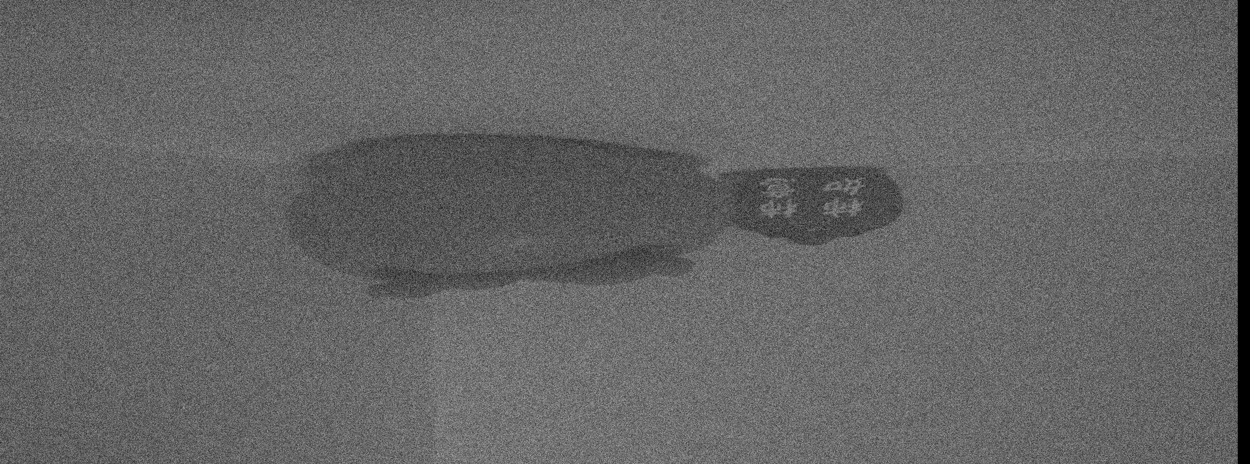
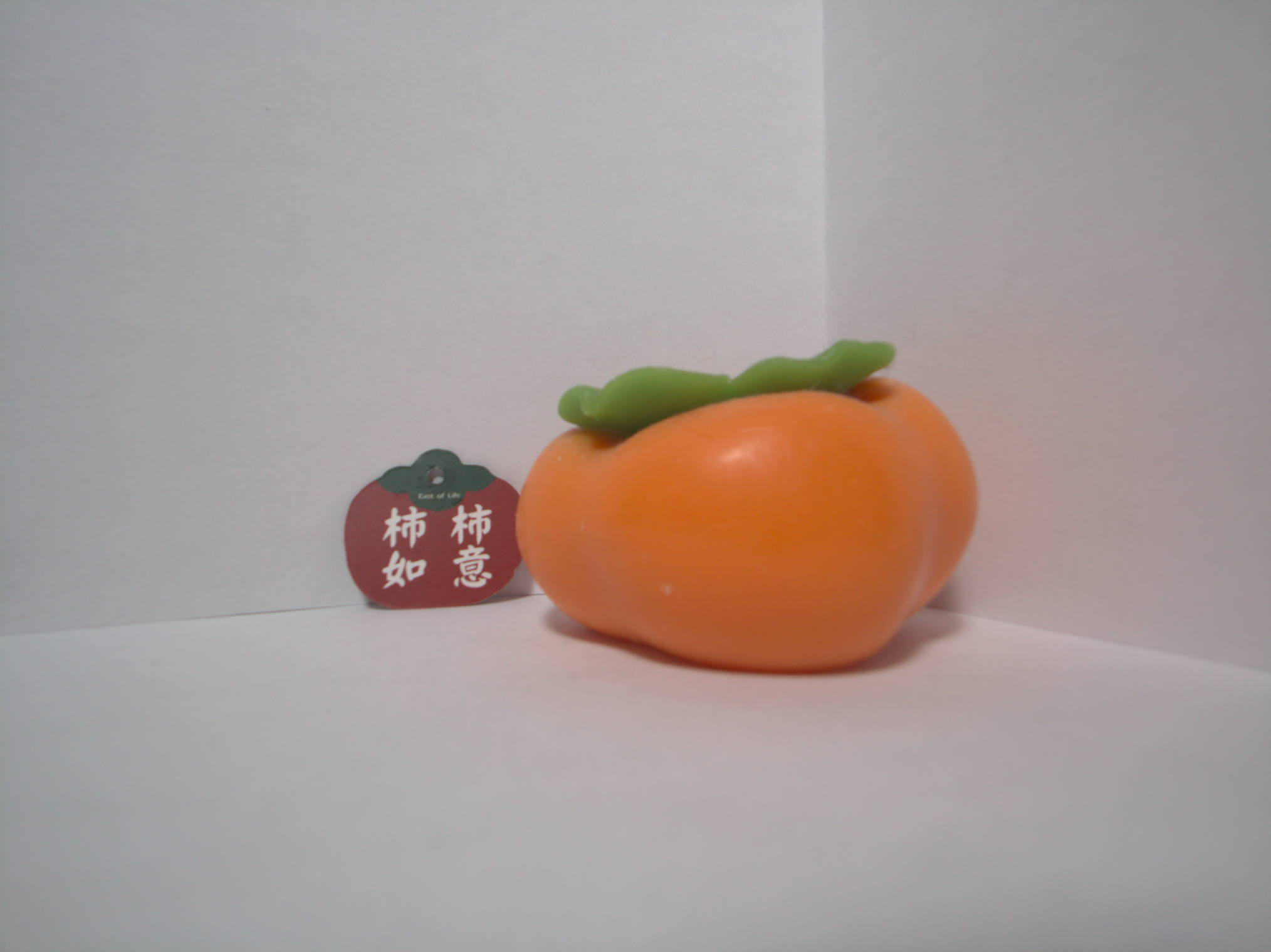
By developing this ISP from scratch, I have laid the foundation for a DIY stereo vision platform that ensures both image accuracy and geometric integrity—key components for depth estimation and 3D reconstruction. A lightweight Python library for reproducible raw processing is released for others building their own computer vision system (See GitHub). Below is a comparison of the raw Bayer image and the custom real-time ISP-processed raw Bayer images from the Pi HQ Camera:

Raw Bayer image – Pi HQ camera:

Processed Image – custom real-time ISP:

Capturing Raw Bayer Data

I use the Picamera2 library to access raw Bayer frames from the Raspberry Pi HQ camera live. This gives me full control over the raw image data before any automatic processing occurs.

def initialize_camera(camera_id, image_size):
    """
    Initialize a Raspberry Pi camera using Picamera2.

    Args:
        camera_id (int): ID of the camera to use (0 or 1 for CSI port).
        image_size (tuple): Desired image resolution as (width, height), e.g., (2028, 1520).

    Returns:
        picam2: Initialized camera object.
        output_im_size (tuple): Actual image size as (width, height).
    """
    picam2 = Picamera2(camera_id)
    config = picam2.create_preview_configuration(raw={'format': 'SBGGR12', 'size': image_size})
    picam2.configure(config)
    print("Camera configuration:")
    print(picam2.camera_configuration())
    img_width_px, image_height_px = picam2.camera_configuration()['sensor']['output_size']
    picam2.start()
    output_im_size = (img_width_px, image_height_px)
    return picam2, output_im_size

# Example
cam_obj, output_im_size_px = initialize_camera(camera_id=0, image_size=(2028, 1520))
raw_u8 = capture_raw_image(cam_obj)

Reconstructing 16 bit images and Stride Correction

The Raspberry Pi HQ Camera produces 12-bit raw sensor data that is packaged into a 16-bit container. Instead of standard 16-bit raw images, the data is stored in a split 8-bit format, where the two bytes must be combined to recover the original values. Understanding the roles of the Most Significant Byte (MSB) and Least Significant Byte (LSB) is key:

• MSB: The upper 8 bits of a 16-bit number (captures the coarse, higher-order information).
• LSB: The lower 8 bits of a 16-bit number (captures the finer detail).

For example, suppose a pixel’s true value is 0xABCD (hex) = 43981 (decimal).

• MSB = 0xAB = 171 (decimal)
• LSB = 0xCD = 205 (decimal)

When recombined, (MSB « 8) | LSB = 43981. If reduced to 8-bit, dividing by 256 gives int(43981 / 256) = 171, which matches the MSB. In practice, this means the 16-bit value can be approximated in 8-bit form using only the MSB, though with some loss of fine detail.

The camera outputs data in two interleaved 8-bit columns: even columns store the LSB, and odd columns store the MSB. Thus, the raw image has shape (H, 2*W) for an image of height H and width W, where each adjacent pair of columns encodes one 16-bit pixel value. The code snippet below reconstructs the full 16-bit image; if only an 8-bit representation is needed, the MSB alone can be used:

# raw: 8-bit interleaved data (shape: H, 2*W)
lsb = raw_u8[:, ::2].astype(np.uint16)
msb = raw_u8[:, 1::2].astype(np.uint16)
raw16 = (msb << 8) | lsb  # Combine into 16-bit values

raw8 = raw_u8[:, 1::2].astype(np.uint8)

Stride correction

Striding refers to the number of bytes in memory used to store a single row of image data — including any extra padding bytes added after the actual image pixels. Padding is typically introduced so that each row begins at a memory address that is efficient for the hardware to access.

In most imaging systems, the stride is aligned to specific memory boundaries such as 8, 64, 128, or 256 bytes, depending on the hardware’s memory and direct memory access (DMA) requirements. These alignments allow faster memory transfers and simplify address calculations.

For the Raspberry Pi HQ Camera, the raw output is 8-bit per pixel. With 2×2 binning, the image width is 2028 pixels (half of the IMX477 sensor’s 4056 active pixels). Because MSB and LSB values are interleaved, this results in 2028 × 2 = 4056 pixels per row, at 8 bits each.

Thus, one row contains 4056 bytes of pixel data. Since DMA requires the stride to be a multiple of 256, the row length is padded with an additional 40 bytes. This makes the actual stride 4096 bytes per row. The figure below illustrates the interleaved MSB/LSB columns and how striding is applied.

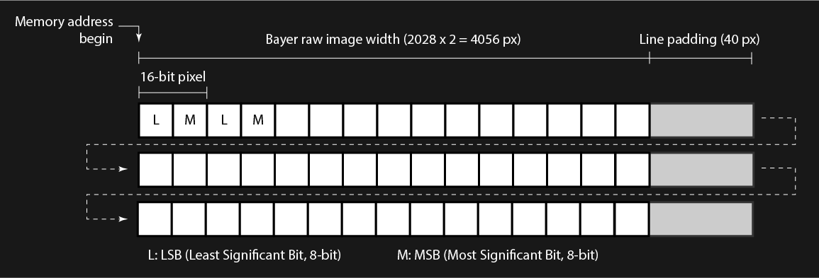
The code below demonstrates how to reconstruct either a 16-bit or 8-bit image with stride correction applied. The figure shows the raw interleaved 8-bit output from the camera alongside the properly reconstructed 16-bit image. Notice the black edge on the right side of the Raw Bayer Image—this corresponds to the 40 padded pixels added at the end of each row.

def unpack_and_trim_raw(raw, img_width_px, bit_depth=16):
    """
    Remove padding or stride artifacts from a raw Bayer image.

    For 16-bit raw images (from Pi HQ camera), the data is packed into two interleaved 
    8-bit columns: the lower 8 bits (LSB, Least Significant Bit) and higher 8 bits (MSB, Most Significant Bit). This function 
    reconstructs the 16-bit image and removes stride artifacts.

    For 8-bit raw images, only stride correction and trimming are applied.

    Args:
        raw (np.ndarray): Raw image array. For 16-bit, shape (H, 2*W) with LSB and MSB interleaved.
        img_width_px (int): Target width (in pixels) after correction.
        bit_depth (int): Bit depth of raw image. Must be 8 or 16.

    Returns:
        np.ndarray: Corrected raw image with shape (H, img_width_px) and dtype uint8 or uint16.
    """
    if bit_depth == 16:
        # Extract LSB and MSB from interleaved columns and reconstruct 16-bit raw
        lsb = raw[:, ::2].astype(np.uint16)
        msb = raw[:, 1::2].astype(np.uint16)
        raw_corrected = (msb << 8) | lsb

    elif bit_depth == 8:
        # For 8-bit data, simply remove padding (if any) and use as-is
        lsb = raw[:, ::2].astype(np.uint16)
        msb = raw[:, 1::2].astype(np.uint16)
        raw_corrected = (msb << 8) | lsb
        # Convert to 8-bit, this is same as (raw_corrected/256).astype('uint8'), but faster. 
        # 65535/256 = 255.99, int (255.99) = 255, 65535 is 2^16 - 1
        raw_corrected = (raw_corrected >> 8).astype('uint8') 

    else:
        raise ValueError("bit_depth must be either 8 or 16")

    # Trim to the exact target width
    raw_corrected = raw_corrected[:, :img_width_px]

    return raw_corrected

Raw Bayer image:

Reconstructed Bayer image:

Black Offset Correction

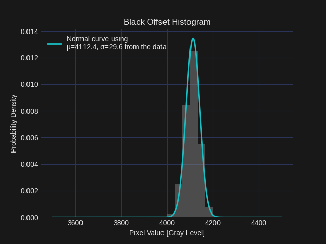
The black offset was characterized with the camera’s optical path completely blocked by a lens cap to ensure no incident light. The analog gain was set to 4.0, corresponding to the midpoint of the Raspberry Pi HQ camera’s gain range (1.0–8.0), and the exposure time was set to 500 µs. This short exposure minimizes the contribution of dark current to the measurement. The black offset is defined here as the mean pixel value, expressed in gray levels (GL), computed over the entire image frame. Under these conditions, the measured black offset was approximately 4110 GL, as shown in the histogram below. This offset is subtracted from all subsequent raw images as part of the preprocessing pipeline. The implementation of the black offset subtraction function is also provided below.

def apply_black_offset(image, offset):
    """
    Subtracts a constant black offset from the image. 
    Offset can be measured from the black_offset_measurement.py script.

    Args:
        image (np.ndarray): Input raw image (can be float or integer type), 8bit or 16 bit image.
        offset (int): The constant black level to subtract.

    Returns:
        np.ndarray (int): Black-offset corrected image (clipped to [0, inf]).
    """
    # Subtract black offset and clip
    corrected = image.astype(np.float32) - offset   #Convert to float to prevent overflow

    if image.dtype == np.uint8:
        corrected = np.clip(corrected, 0, 255).astype(np.uint8)
    elif image.dtype == np.uint16:
        corrected = np.clip(corrected, 0, 65535).astype(np.uint16)

    return corrected

# Example
raw_unstrided_blckoff_u16 = apply_black_offset(raw_u16, offset=4110)

Demosaicing

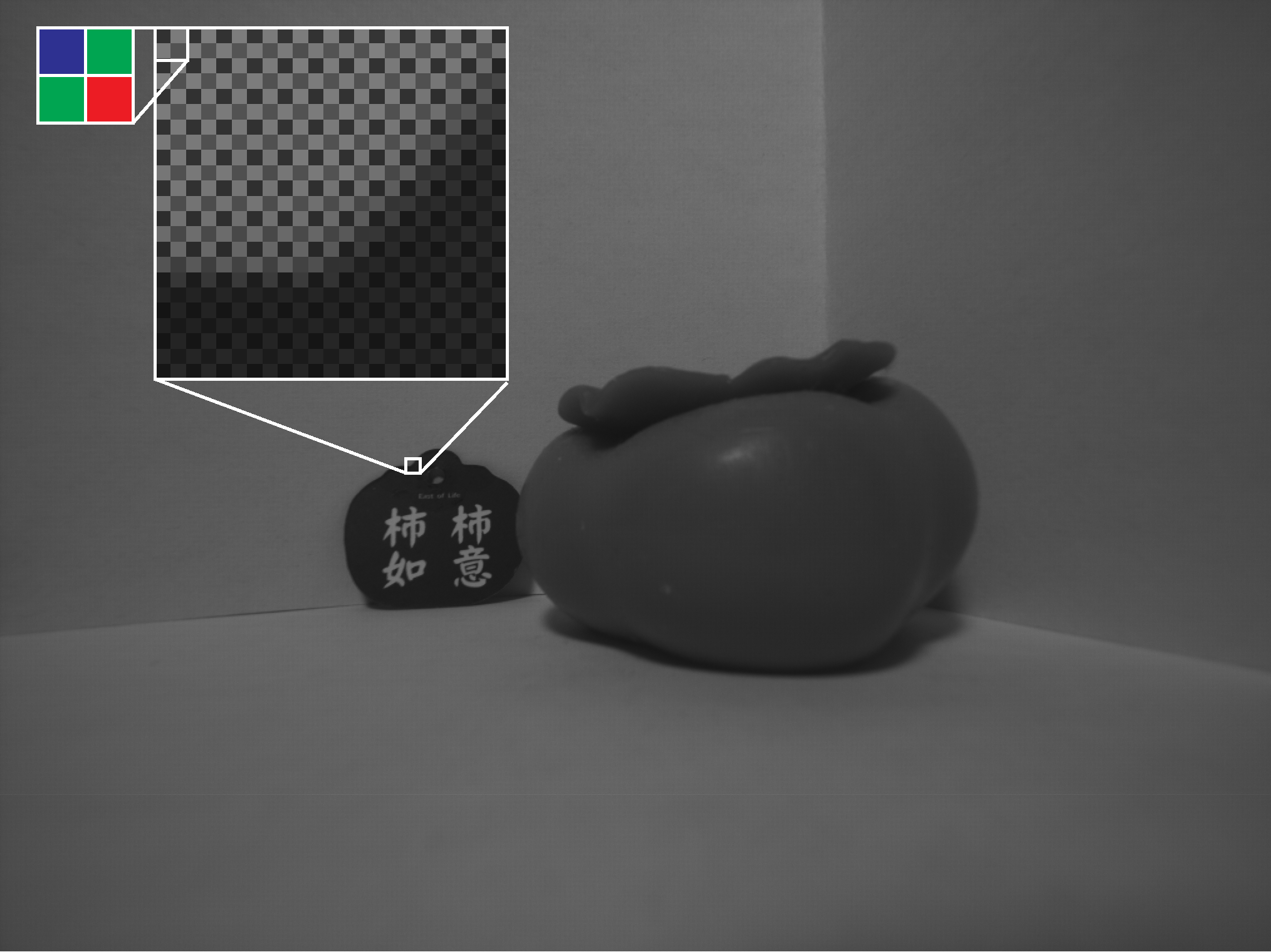
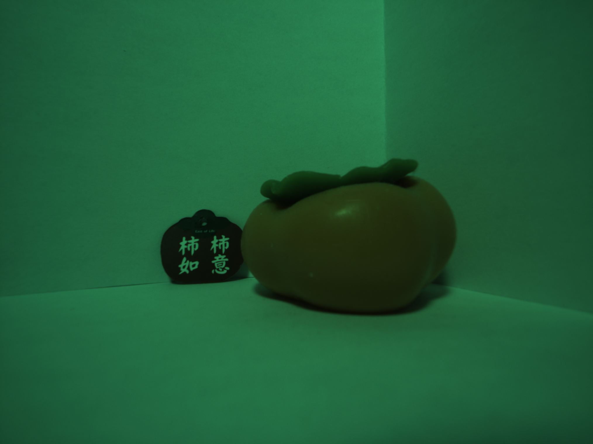
A simple bilinear demosaicing algorithm from the OpenCV library is used to convert the Bayer image into a three-channel RGB image. In bilinear demosaicing, each missing color value is estimated by averaging the nearest four pixels of that color channel. The figure below compares the linear image before and after demosaicing. For visual reference, the Bayer mosaic pattern used here is BGGR, as shown in the inserted diagram. Note that the images are presented in linear RGB space (with no gamma encoding applied). While bilinear interpolation is straightforward, there are many more advanced demosaicing algorithms that can produce higher-quality results. The implications of different demosaicing choices will be discussed in the next blog post.

linear_bgr = cv2.cvtColor(raw_unstrided_blckoff_u16, cv2.COLOR_BAYER_BGGR2BGR)

Raw Bayer image:

Demosaic image:

White Balance Using a Gray Neutral Patch

To ensure accurate color reproduction—making white in the scene appear white under the scene’s lighting conditions, or making a gray patch render as gray, i.e. \(R \approx G \approx B\), I calibrated and applied per-channel gains (white balance) using a known neutral patch in the scene.

Let the measured RGB values of the patch from the captured image and the reference (grouth truth) values be:

The gain per each color channel are:

I then normalize so that the mean of the all gains is 1:

Since no perfectly neutral gray patch was available, I selected the most neutral patch from the SpyderCHECKR chart, with sRGB values of [80,80,78]. The implications of this choice will be discussed in the next post. The images below show the scene before and after white balance. Both are gamma-encoded to sRGB for correct display, the white balance calculations themselves were done in linear RGB space.

Demosaic image:

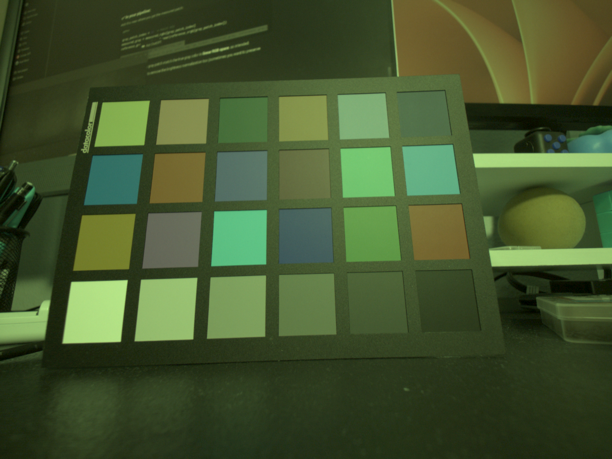
Image after white balance:

def white_balance_to_gray_patch(img_rgb_f01, measured_patch_rgb_f01, reference_patch_rgb_f01):
    """
    Applies white balance correction based on a reference gray patch.

    The function computes per-channel gains so that the measured RGB value of a gray patch
    matches a given reference value. The correction is applied globally to the image, and
    the gains are normalized so that the mean channel gain is fixed at 1.0.

    Args:
        img_rgb_f01 (np.ndarray): Input image in linear RGB, float32/float64, values in [0, 1].
                                  Shape (H, W, 3).
        measured_patch_rgb_f01 (np.ndarray): Measured average RGB value of the gray patch,
                                             shape (3,), float, in [0, 1].
        reference_patch_rgb_f01 (np.ndarray): Target RGB value for the gray patch,
                                              shape (3,), float, in [0, 1].

    Returns:
        tuple:
            np.ndarray: White-balanced image, same shape as input, clipped to [0, 1].
            np.ndarray: Per-channel gains applied (R, G, B).
    """
    # Compute per-channel gains (avoid divide-by-zero with np.clip)
    wb_gains = reference_patch_rgb_f01 / np.clip(measured_patch_rgb_f01, 1e-6, None)

    # Normalize so that the average of R, G, B gains is 1
    wb_gains = wb_gains / wb_gains.mean()

    print(f"White balance gains: {wb_gains}")

    # Apply gains to image
    img_wb_f01 = img_rgb_f01 * wb_gains

    # Rescale if any values exceed 1.0
    max_val = img_wb_f01.max()
    if max_val > 1.0:
        img_wb_f01 /= max_val

    return np.clip(img_wb_f01, 0, 1), wb_gains

Color Correction Matrix (CCM)

After white balance, a 3×3 Color Correction Matrix (CCM) is applied to map the camera’s linear RGB values to a target color space. The CCM is estimated using a least-squares fit between the 24 measured patch colors from the captured chart and the corresponding ground-truth patch values.

Each measured patch value is multiplied by the CCM to produce its corrected color, minimizing overall color error across all patches. This step compensates for the sensor’s spectral sensitivity and lens transmission characteristics, allowing the rendered colors to more closely match their true appearance. The correction is performed entirely in the linear domain, and the correction result is gamma-encoded to sRGB for display.

Using the measured RGB values from the 24 color patches and their known ground-truth values (in linear RGB), the CCM is solved via least squares.

Let:

We solve for the 3×3 Color Correction Matrix \(\mathbf{A}\) such that

The least-squares solution is

Once \(\mathbf{A}\) is found, each pixel of the white-balanced image \(\mathbf{I}_{\text{measured}}\) can be color corrected as:

Here, the first column of \(A\) controls how much of the input (R, G, B) contributes to the corrected R channel; the second column controls the contributions to corrected G; and the third column controls contributions to corrected B. In other words, each corrected RGB channels is formed as a linear mix of the input RGB channels. This can be thought of as “color mixing” for each pixel, adjusting the camera’s raw response so that the rendered colors align with the ground-truth values of the ColorChecker patches.

For this calibration, the chart was illuminated by a D50, 5000K, CRI 90, anti-flicker light bulb. While reasonably neutral, such light sources can still introduce small errors because their spectral power distribution differs from a true reference illuminant. In color science, the true references are the CIE Standard Illuminants (e.g., D65, 6500 K, which defines the white point of sRGB). These standardized spectra provide the benchmark for accurate color reproduction. The implications of using a D50 light bulb instead of a standard illuminant will be discussed in the next blog post.

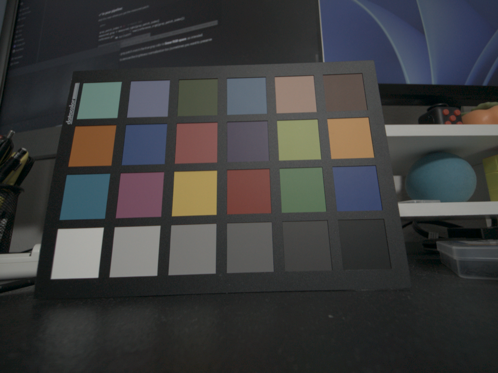
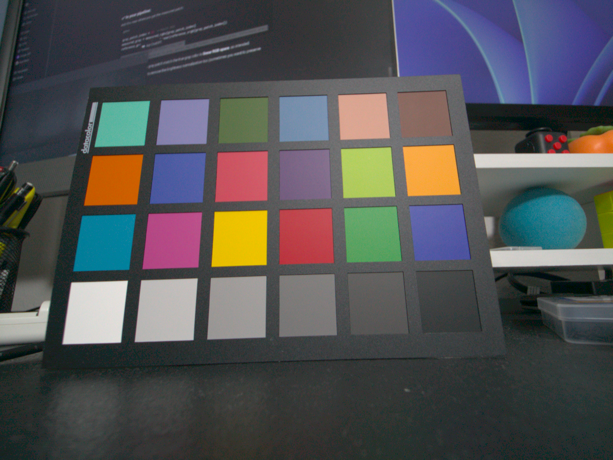
Image after white balance (gamma-encoded for display):

Image after color correction (gamma-encoded for display):

def srgb_to_linear(srgb_f01: np.ndarray) -> np.ndarray:
    """
    Convert sRGB to linear RGB (IEC 61966-2-1 standard).

    Parameters
    ----------
    srgb_f01 : np.ndarray
        sRGB image or array with values in [0, 1].

    Returns
    -------
    linear : np.ndarray
        Linear RGB image or array with values in [0, 1].
    """
    srgb = np.clip(srgb_f01, 0.0, 1.0)
    linear = np.where(
        srgb <= 0.04045,
        srgb / 12.92,
        ((srgb + 0.055) / 1.055) ** 2.4
    )
    return np.clip(linear, 0.0, 1.0)

# Ground-truth SpyderCHECKR patch colors (sRGB in [0,1])
ground_truth_patches_srgb_f01 = (np.array([
    [98, 187, 166], [126, 125, 174], [82, 106, 60], [87, 120, 155], [197, 145, 125], [112, 76, 60],
    [222, 118, 32], [58, 88, 159], [195, 79, 95], [83, 58, 106], [157, 188, 54], [238, 158, 25],
    [0, 127, 159], [192, 75, 145], [245, 205, 0], [186, 26, 51], [57, 146, 64], [25, 55, 135],
    [249, 242, 238], [202, 198, 195], [161, 157, 154], [122, 118, 116], [80, 80, 78], [43, 41, 43]
], dtype=np.float32) / 255.0)

# Convert reference patches to linear RGB
ground_truth_patches_linear_rgb_f01 = srgb_to_linear(ground_truth_patches_srgb_f01)

# --- Solve for 3×3 Color Correction Matrix (CCM) ---
# Least squares: measured @ A ≈ reference
A, _, _, _ = np.linalg.lstsq(
    measured_patches_rgb_linear_f01 * wb_gains,   # shape (24,3), linear, after WB, 24 patches
    ground_truth_patches_linear_rgb_f01,           # shape (24,3), linear
)

# --- Apply CCM to a white balanced image (still in linear) ---
H, W, _ = img_rgb_wb_linear_f01.shape
img_lin = img_rgb_wb_linear_f01.reshape(-1, 3)

corrected_lin = img_lin @ A
corrected_lin = corrected_lin.reshape(H, W, 3)

Gamma Correction to sRGB

After white balance and color correction, the image is still represented in linear RGB. To make it suitable for display, I apply gamma correction to map the linear values into the sRGB color space using IEC 61966-2-1 standard. This step ensures that brightness and contrast appear natural to the human eye, since human vision is non-linear, and also matches the expectations of most displays and file formats.

def linear_to_srgb(linear_rgb):
    """
    Convert linear RGB to sRGB (IEC 61966-2-1 gamma encoding).

    Args:
        linear_rgb (np.ndarray): Image or array in linear RGB with values in [0, 1].
                                 Shape (..., 3). dtype float recommended.

    Returns:
        np.ndarray: sRGB-encoded image/array with values in [0, 1], same shape as input.

    Notes:
        Piecewise transfer function:
          if x <= 0.0031308:  f(x) = 12.92 * x
          else:               f(x) = 1.055 * x^(1/2.4) - 0.055
    """
    linear_rgb = np.clip(linear_rgb, 0, 1)  # Clamp to valid range

    threshold = 0.0031308
    a = 0.055

    srgb = np.where(
        linear_rgb <= threshold,
        linear_rgb * 12.92,
        (1 + a) * np.power(linear_rgb, 1 / 2.4) - a
    )
    return np.clip(srgb, 0, 1)

# Example, applying gamma correction for display
img_rgb_wb_ccm_srgb_f01 = linear_to_srgb(img_rgb_wb_ccm_linear_f01)
img_corrected_u8 = normalize01_to_8bit(img_rgb_wb_ccm_srgb_f01)  # Convert to 8-bit for saving/display

Linear image (before gamma):

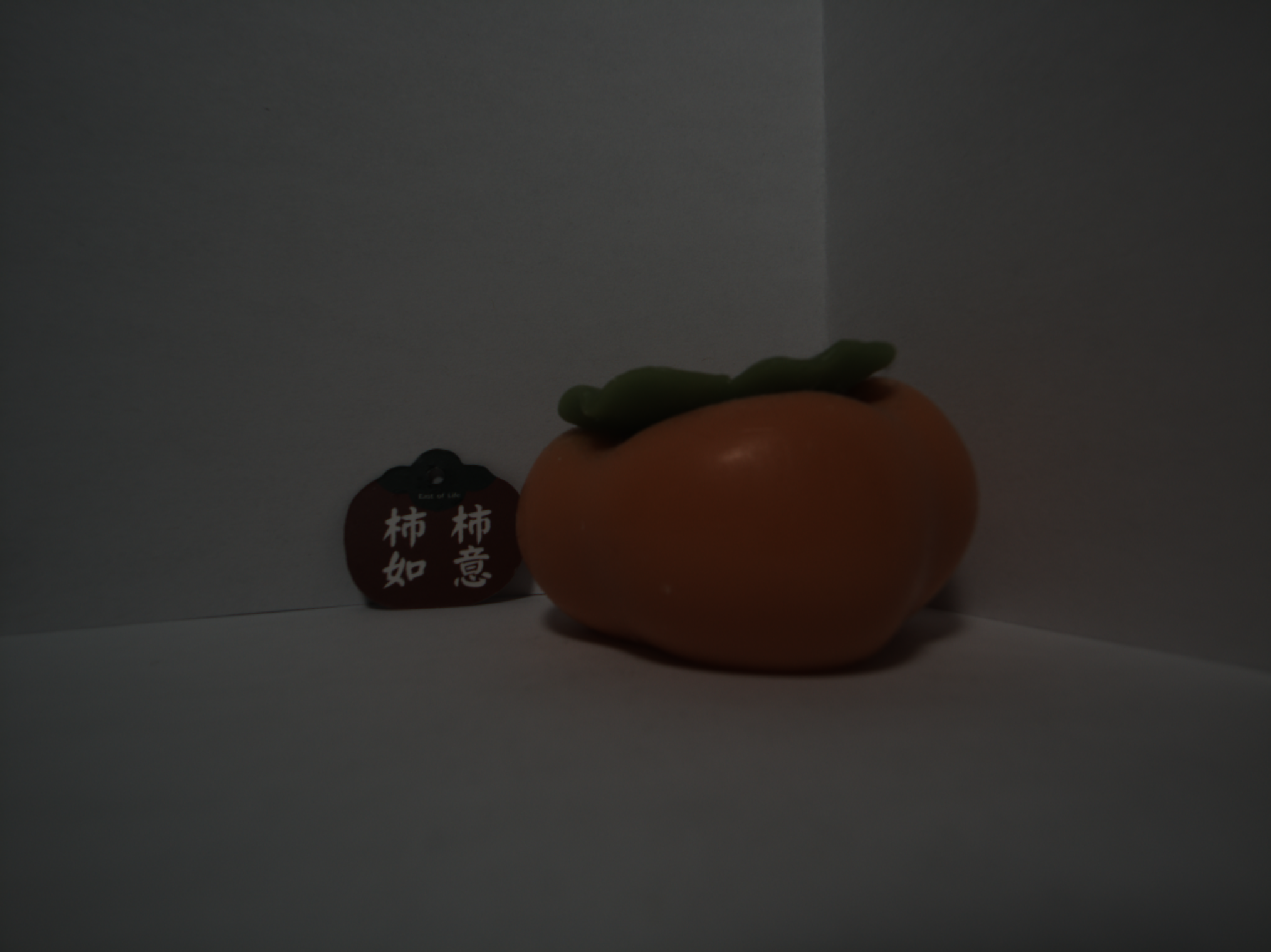
Gamma-corrected sRGB image (for display):

Final Thoughts

This custom ISP pipeline gave me complete control over every step of the imaging process — from raw Bayer capture to final gamma-encoded sRGB output. That level of control is essential for debugging, calibration, and understanding how each stage affects the final image. It also provides a solid foundation for more advanced work, such as stereo vision and high-dynamic-range imaging.

That said, several sources of error remain to be addressed. In this post I used the most neutral patch available on the SpyderCHECKR chart for white balance; because it is not a true gray patch, it introduces bias. Likewise, the Color Correction Matrix was calibrated under a 5000 K, CRI-90 light bulb—reasonable, but not a true reference illuminant like CIE D65 (the sRGB white point)—so absolute color accuracy is affected. In addition, I used simple bilinear demosaicing for clarity; higher-performing methods can reduce zippering, moiré, and color aliasing and will likely improve results. I will dig into these error sources—gray-patch choice, illuminant standards, and demosaicing algorithm selection—in the next blog post.

Other corrections — such as lens shading and distortion correction — were not included here. With a low-distortion lens, these effects are not visually obvious for single-camera use, but they become critical when moving to a stereo setup where geometric precision directly impacts depth accuracy. These corrections will therefore be part of the upcoming stereo camera pipeline.

This pipeline is the beginning. By building everything from scratch, we now have a transparent and customizable imaging system that can evolve toward:

• Per-channel lens shading correction
• Geometric distortion correction
• Real-time performance optimization
• Integration into a stereo depth camera

The next step is to extend this single-camera ISP to a calibrated stereo camera system — the real motivation behind this work.

Stay tuned!