Light Detection and Ranging (LiDAR)

In my last blog post, I discussed optical Time-of-Flight (ToF) sensing and explained how it works with a single emitter that produces a single beam of light and a single-pixel detector. Because of this setup, we could measure the ToF at only one point in space.
The question, then, is: How can we sense depth across an entire area? The answer lies in Light Detection and Ranging (LiDAR) — a system based on ToF that can measure depth over a broad region. In this blog post, I will (a) discuss the fundamentals of LiDAR and (b) demonstrate the optical system of a specific type of LiDAR, Flash LiDAR, using Zemax.
How to scan an area?
To obtain depth information over an area, we need to deliver light across the entire scene. Broadly, there are two main approaches: (1) Mechanical scanning of a single beam across the scene. (2) Wide-field illumination of the scene.
(1) Mechanical Scanning
In mechanical scanning, a single beam is swept across the scene using a mechanical scanner. This is done via raster scanning, where the beam moves horizontally (left to right or right to left), then moves down one line, and repeats until the entire field is covered. The illustration below shows the concept:

Numerous scanning methods can achieve this. The table below lists several scanning technologies, along with the typical speed (line rate) and maximum achievable scanning angle for each. To perform 2D scanning, one can pair two scanning methods (identical or different), depending on specific design criteria. Note that for a given scanning method, increasing speed usually reduces the maximum scanning angle.
| Scanning Method | Line rate | Optical scanning angle | Common Applications |
|---|---|---|---|
| Galvo-mirrors | < kHz | 10o-40o | |
| Resonant-mirrors | ~10 kHz | 1o-15o | |
| Polygon mirror | ~10-100 kHz | 90o-360o | Automative LiDAR |
| MEMS | ~10-50 kHz | 1o-10o | AR/VR headsets, smartphones, compact devices |
| Fiber optics | ~1 MHz | 5o-30o | |
| Rotating mirror | 10-100 Hz | 90o-360o | Automative LiDAR |
| Optical Phased Array (OPA) | ~ MHz | 10o-120o |
(2) Wide-field illumination
In wide-field illumination, the entire scene is illuminated at once, eliminating the need for mechanical scanning. This approach is sometimes called Flash LiDAR. It is used in Apple’s iPhone and iPad LiDAR modules (see image below):
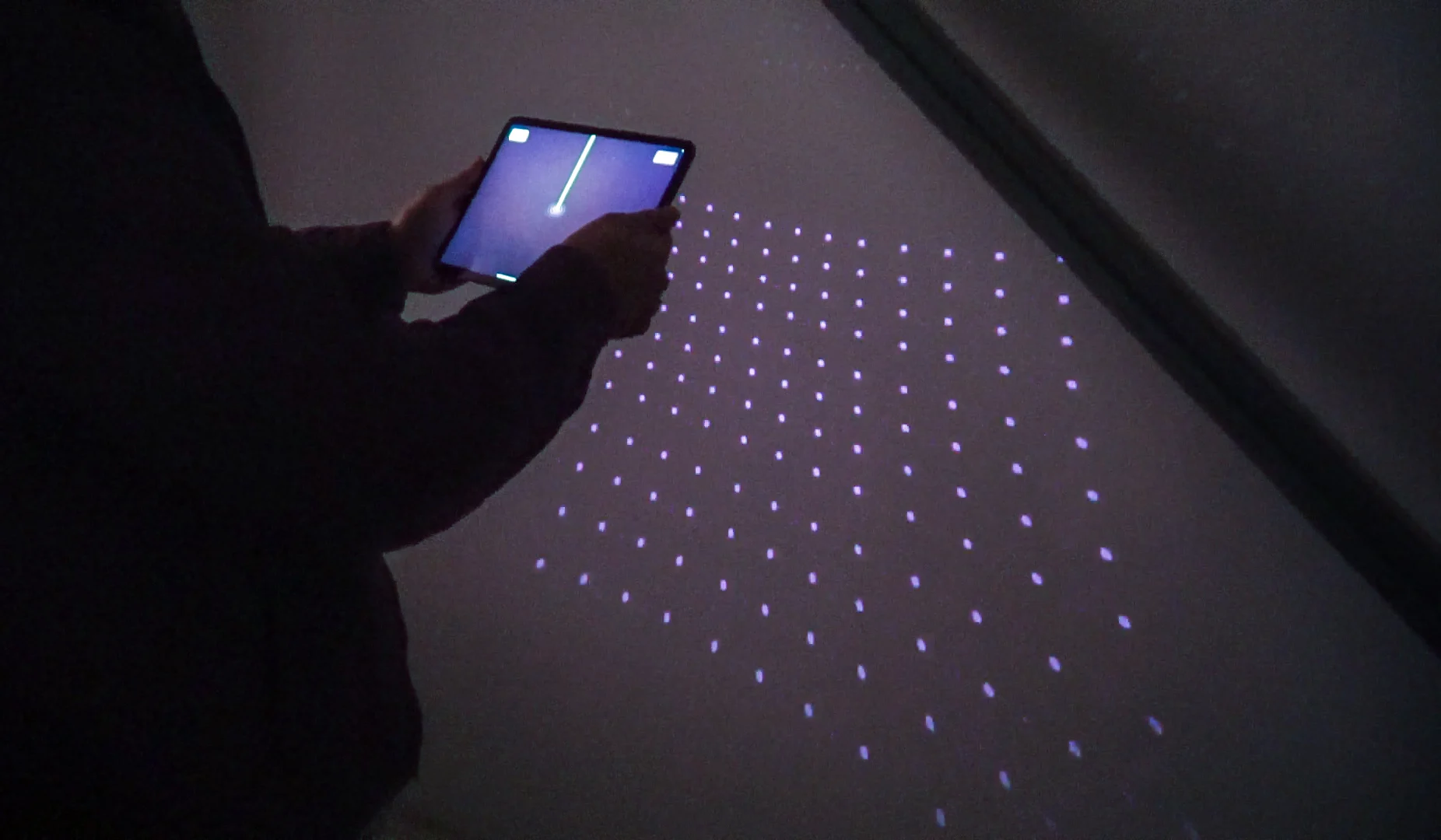
Image from Magicplan.app
This is not to be confused with the Face ID depth-sensing technology, which uses “light coding”. In this post, we focus on ToF-based depth sensing.
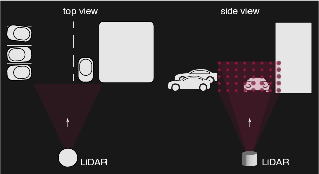
The schematic below illustrates the principle. We flood the entire scene with light (usually infrared), then capture the reflected or scattered light on a sensor (e.g., Sony IMX591). The depth for the entire scene is determined in a single shot—akin to a camera flash—thus the name Flash LiDAR.
Flash LiDAR illumination typically uses VCSEL (Vertical Cavity Surface-Emitting Laser) arrays that emit short pulses (on the order of nanoseconds) and form dot patterns. Temporal (pulsing) and spatial (dot pattern) modulation both help improve the signal-to-noise ratio (SNR). We’ll cover more details in a separate post. Briefly, pulsed lasers enable temporal separation of the laser signal from ambient light and dot patterns enable spatial separation of the laser signal from ambient light. For ToF detection, avalanche photodiodes (APDs) or silicon photomultipliers (SiPMs) measure the ToF of the laser pulses directly, typically with resolutions on the order of hundreds of picoseconds. These photodiodes are arranged in a 2D array to capture the entire scene’s depth information simultaneously, just like a camera sensor.
Simulation of flash LiDAR optical system
Illumination system
A key goal in Flash LiDAR illumination is to project a dot-pattern over the target area. Below is an example of a VCSEL array as the light source:
Image from lighttrans.com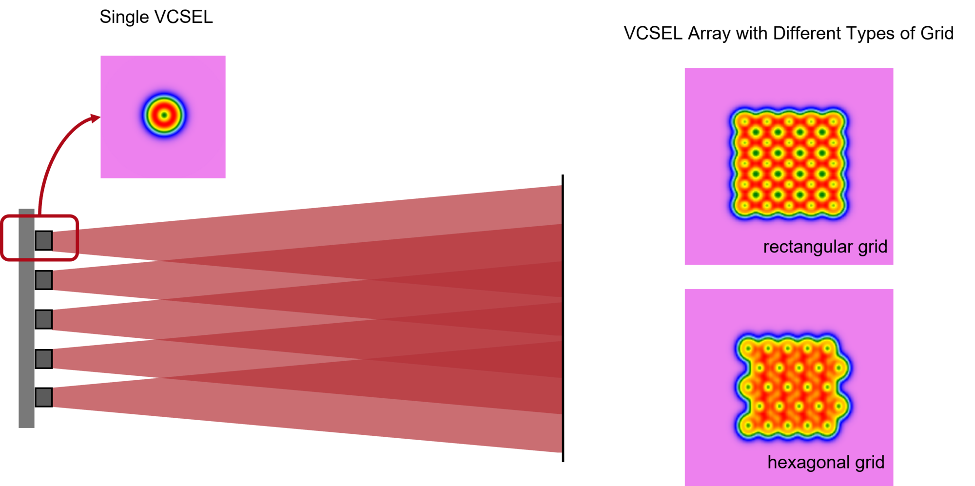
Our aim is to project the 1.6 × 1.6 mm square source to approximately a 160 × 160 mm area at 1 m from the last lens surface. This can be achieved using an aspheric collimating lens of fixed focal length.
Using the thin-lens equation,
\[\frac{1}{f} = \frac{1}{d_o} + \frac{1}{d_i}\]where:
- \(f\) is focal length of the lens
- \(d_o\) is the object distance
- \(d_i\) is the image distance
and the magnification relation,
\[M = \frac{d_i}{d_o} = \frac{h_i}{h_o}\]where:
- \(h_o\) is the object height
- \(h_i\) is the image height
- \(M\) is magnification of the lens
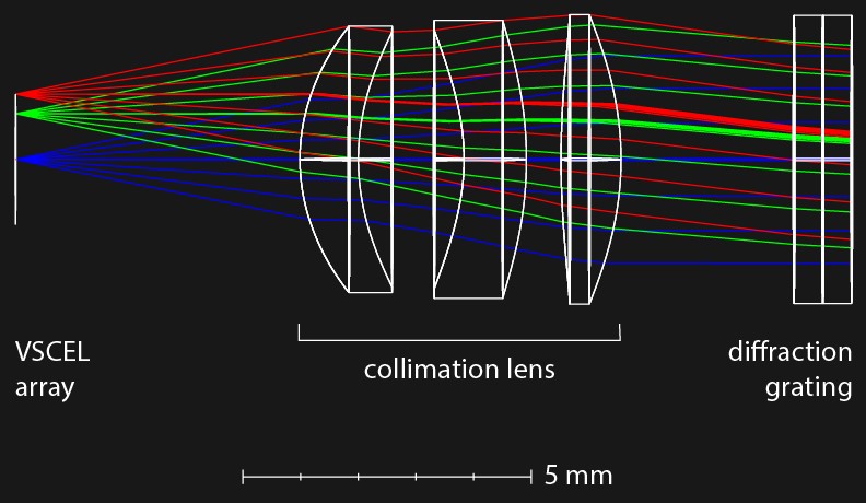
We find that a focal length \(f\) of 10 mm is needed. The collimator below shows the lens we need. The VCSEL array will be placed at the object plane. The object plane in the Zemax model is about 2.26 mm diagonally — this corresponds to the diagonal of a 1.6 mm square that the optical design must accommodate.
Lenses from Zemax.com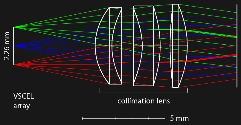
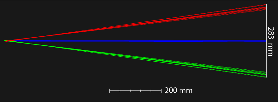
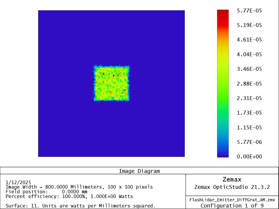
Using Zemax, we can visualize the intensity distribution from the 1.6 × 1.6 mm square at the image plane, which is roughly 200 mm × 200 mm (the diagonal is about 283 mm):
If 283 mm of illumination is insufficient, we can add two diffraction gratings oriented perpendicularly to expand the illumination Field of View (FOV). The images below show the effect of these gratings. Notice that higher-order diffraction patterns become distorted because the diffraction angle depends on the incidence angle. Different points on the VCSEL array hit the grating at slightly different angles, leading to different diffraction angle.
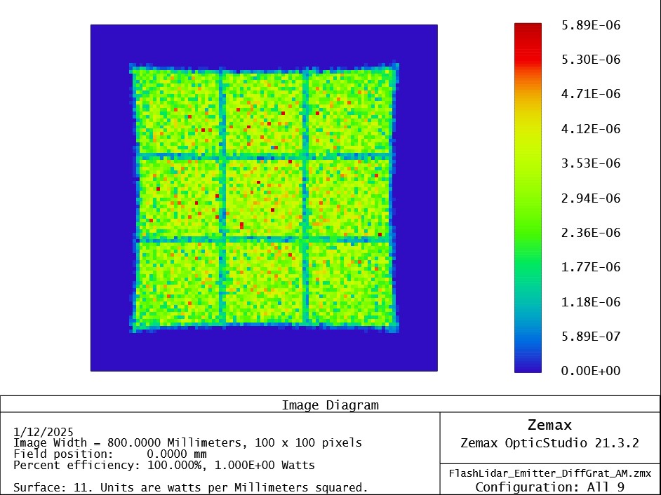
Here, we show the intensity distribution of the whole FOV. However, if the object plane is a VCSEL array, the final projected pattern is a grid of dots. The iPhone LiDAR pattern below illustrates how Apple uses a VCSEL array and diffraction gratings for the flash LiDAR system:
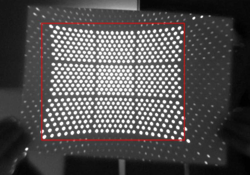
Image from medium.com
Imaging system
The Flash LiDAR imaging system is to capture the projected dot pattern scattered from objects in the environment. This imaging system must: (1) Have a large enough FOV to capture all the dots in the pattern and (2) provide sufficient contrast to resolve each dot.
With the crossed diffraction gratings, we expanded the illumination FOV to a 600 × 600 mm area at 1 m (i.e., 3 × 200 mm). The half-FOV required for the imaging system then becomes:
\[tan (\theta_{FOV}) = \frac{424 mm}{1000 mm} \Rightarrow \theta_{FOV} = 23^o\]The 424 mm is the half diagonal of the 600 x 600 mm square. We can image this FOV with a common Cooke triplet imaging lens—essentially a high-index negative lens sandwiched between two low-index positive lenses:
Lenses from Zemax.com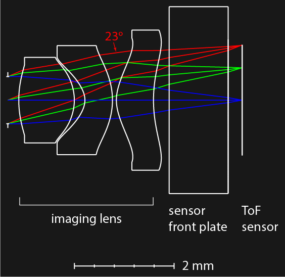
Simulating the optical performance at a 23° FOV shows that it approaches diffraction-limited quality:
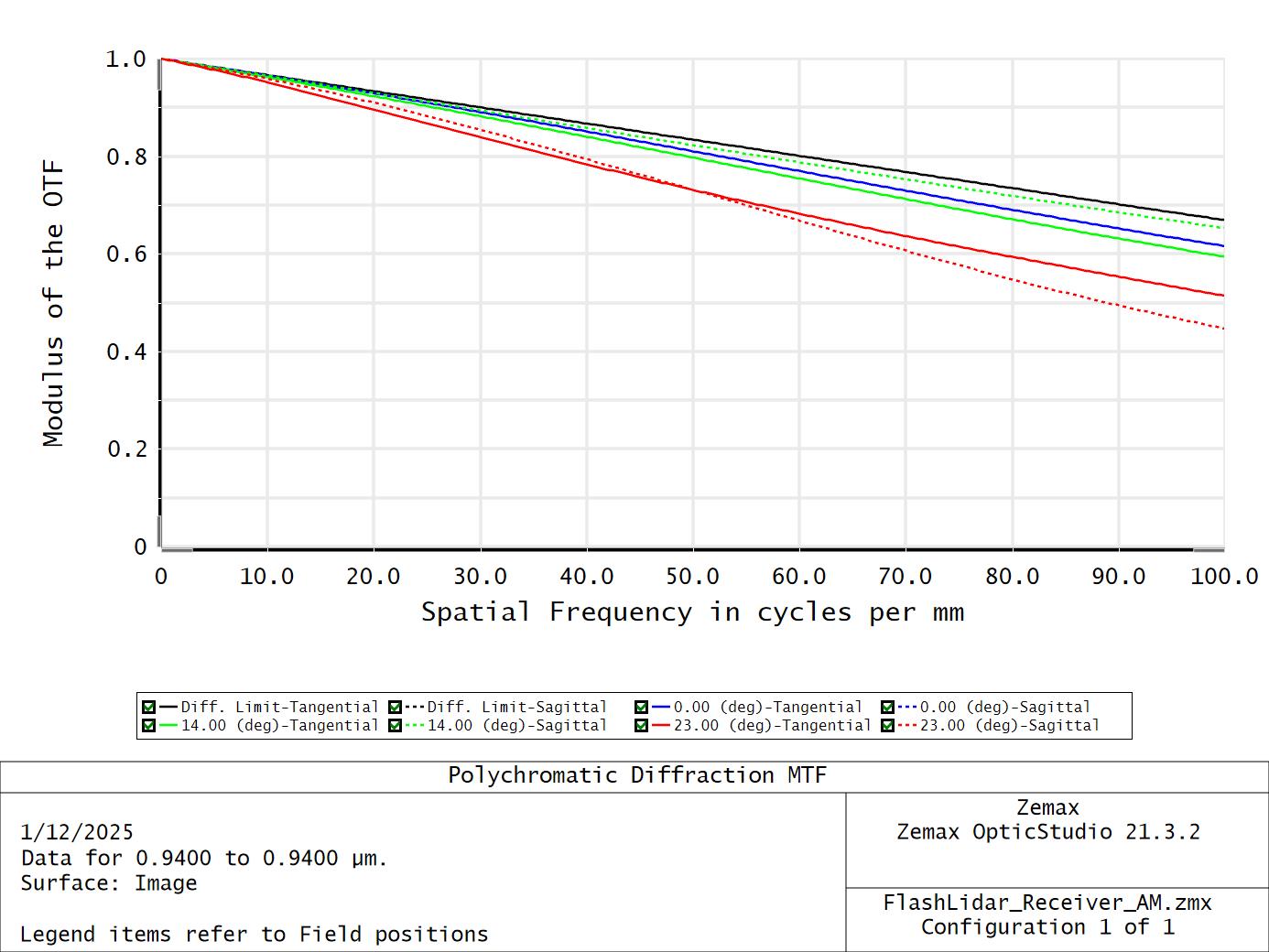
In summary, by combining dot-pattern illumination (Flash LiDAR) with a suitably designed imaging lens, we can capture depth information of an entire scene in one shot. Combined with a ToF sensor, we can achieve a truly camera-like Tof depth measurement system.
Reference
- https://blog.magicplan.app/why-apples-lidar-scanner-opens-up-a-brave-new-world-of-indoor-mapping
- https://support.zemax.com/hc/en-us/articles/4408930472467-Modeling-a-Flash-Lidar-System-Part-1
- https://www.lighttrans.com/index.php?id=2573&utm_source=newsletter&utm_medium
- https://4sense.medium.com/lidar-apple-lidar-and-dtof-analysis-cc18056ec41a
- Padmanabhan, P., Zhang, C., & Charbon, E. (2019). Modeling and analysis of a direct time-of-flight sensor architecture for LiDAR applications. Sensors, 19(24), 5464.
- Nayar, S. K., Krishnan, G., Grossberg, M. D., & Raskar, R. (2006). Fast separation of direct and global components of a scene using high frequency illumination. In ACM SIGGRAPH 2006 Papers (pp. 935-944).