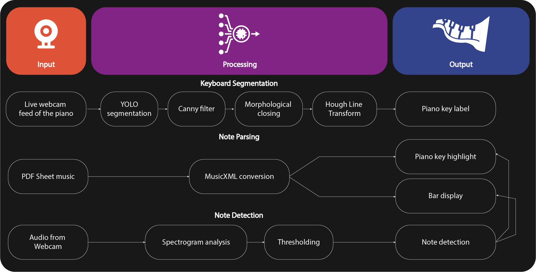
My AI Piano Tutor

ToF art

I am a beginner piano player—despite holding ABRSM Grade 8 in both oboe and music theory. Piano presents a new set of challenges. For me, the difficulty lies in sight-reading: identifying notes on both clefs, finding the correct keys on the keyboard, and coordinating both hands in real time. That became the inspiration for this project: building my own AI-powered piano tutor using computer vision, a webcam, and a piano to improve my sight-reading.

As an oboist, I am used to instinctively translating notes into fingerings. That gave me an idea: what if I could use a webcam and computer vision to detect the piano keys, label them, and show me which key to press next? This kind of real-time mapping between sheet music and hand movement might help build muscle memory and improve sight-reading over time.

In this project, I demonstrate how I use a webcam and computer vision to identify individual piano keys in real time, display which key to press based on sheet music, and detect which notes are actually played using audio.

Flow chat of the whole process

The diagram below summarizes the full workflow.

Section 1: Keyboard segmentation

To detect individual keys in real time—even when hands are partially covering the keyboard—I implemented a hand removal step. When hands are detected using MediaPipe, the corresponding regions are replaced with a clean reference image. Since the keyboard position is fixed relative to the camera, users also have the option to lock on the key labelling. This prevents instability caused by occlusion during hand movement.

import mediapipe as mp
hands = mp.solutions.hands.Hands(static_image_mode=False, max_num_hands=2, min_detection_confidence=0.7)
results_hands = hands.process(frame_rgb)
for hand_landmarks in results_hands.multi_hand_landmarks:
    xs = [int(landmark.x * w_img) for landmark in hand_landmarks.landmark]
    ys = [int(landmark.y * h_img) for landmark in hand_landmarks.landmark]
    x_min, x_max = max(min(xs) - 20, 0), min(max(xs) + 20, w_img)
    y_min, y_max = max(min(ys) - 20, 0), min(max(ys) + 20, h_img)

    # Replace the hand area with pixels from the clean reference
    clean_reference_matched = self.match_brightness(frame, self.clean_reference)
    frame[y_min:y_max, x_min:x_max] = clean_reference_matched[y_min:y_max, x_min:x_max]

Example result:

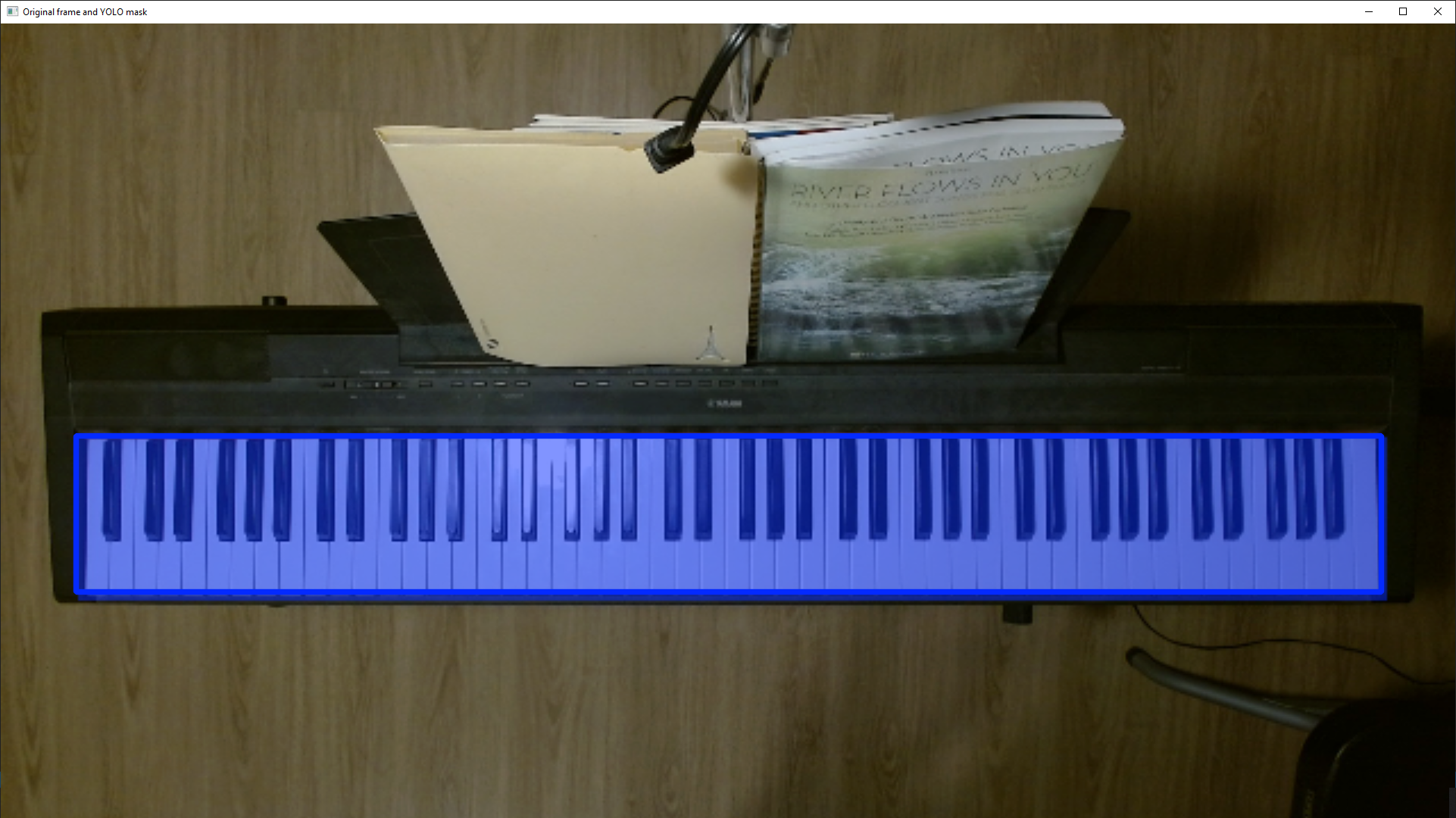
YOLOv8 segmentation

I trained a YOLOv8 segmentation model using a dataset of 572 piano images from Roboflow (dataset link). The example below shows the segmentation result, along with the code used to train and apply the model.

from ultralytics import YOLO
# Load a YOLOv8 segmentation model (you can start with a pretrained one)
model = YOLO("yolov8n-seg.pt")  # or yolov8s-seg.pt, yolov8m-seg.pt, etc.
# Train the model
model.train(
    data="piano_dataset/data.yaml",  # path to dataset config from Roboflow export
    epochs=50,
    imgsz=640,
    batch=8,
    project="piano_seg_yolov8",
    name="train",
    task="segment"
)

model = YOLO("piano_seg_yolov8/runs/segment/train2/weights/best.pt")
results = model(frame, conf=0.9)[0]
yolo_mask = results.masks.data[0].cpu().numpy()
yolo_mask = cv2.resize(yolo_mask, (frame.shape[1], frame.shape[0]))
yolo_mask = (yolo_mask * 255).astype(np.uint8)
_, binary_mask = cv2.threshold(yolo_mask, 128, 255, cv2.THRESH_BINARY)
x, y, w, h = cv2.boundingRect(binary_mask)

Edge Detection & Morphology

Next, I applied CLAHE equalization to make the white key gaps stand out more. This method works well even under uneven lighting conditions. Canny edge detection highlight vertical edges of white keys. Then, a morphological closing operation fills small gaps in the edge detection result.

h = piano.shape[0]
white_keys = piano[int(h * 0.7):]  # bottom quarter

clahe = cv2.createCLAHE(clipLimit=3.0, tileGridSize=(8,8))
equalized_white_keys = clahe.apply(white_keys)
cv2.imshow("Equalized white keys", equalized_white_keys)

white_key_edges = cv2.Canny(equalized_white_keys, 50, 150, apertureSize=3)
kernel = np.ones((3, 3), np.uint8)
closed_edge = cv2.morphologyEx(white_key_edges, cv2.MORPH_CLOSE, kernel)
cv2.imshow("Edge detection", white_key_edges)
cv2.imshow("Closed edge detection", closed_edge)

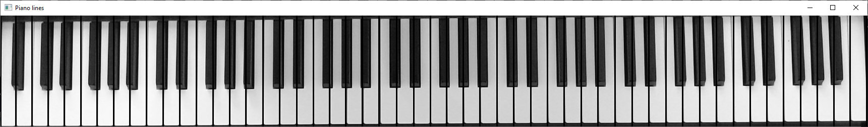
Hough Line Transform

Using the processed edge map, I applied a probabilistic Hough transform to detect mostly vertical lines between white keys. These were then stabilized across frames and merged.

# Detect line segments using the Probabilistic Hough Transform
lines = cv2.HoughLinesP(
    closed_edge,           # Edge-detected binary image
    rho=1,                 # Distance resolution in pixels
    theta=np.pi / 180,     # Angle resolution in radians (1 degree)
    threshold=10,          # Minimum number of votes (intersections in Hough grid)
    minLineLength=20,      # Minimum length of line to be accepted
    maxLineGap=10          # Maximum allowed gap between line segments to treat them as a single line
)

vertical_lines = []                   # Store vertical line segments
line_img = white_keys.copy()          # Copy image for visualizing detected lines

# If lines are detected
if lines is not None:
    for line in lines:
        x_1, y_1, x_2, y_2 = line[0]   # Extract endpoints
        angle = np.arctan2((y_2 - y_1), (x_2 - x_1)) * 180 / np.pi  # Calculate angle of the line in degrees

        # Filter out non-vertical lines (keep lines near 90°)
        if abs(angle) > 80:
            cv2.line(line_img, (x_1, y_1), (x_2, y_2), (0, 0, 0), 2)
            vertical_lines.append((x_1, y_1, x_2, y_2))                 # Save vertical line

# Calculate x-coordinate of the center of each detected vertical line
frame_x_centers = [int((x_1 + x_2) / 2) for (x_1, y_1, x_2, y_2) in vertical_lines]
frame_x_centers.sort()  # Sort from left to right

merged_xs = []  # List of merged and stabilized x-positions

# Add current frame's x-centers to the buffer
line_buffer.append(frame_x_centers)
if len(line_buffer) > buffer_size:
    line_buffer.pop(0)  # Maintain fixed buffer size

# Once enough frames are buffered, merge x-coordinates for temporal smoothing
if len(line_buffer) == buffer_size:
    # Flatten all x-centers across buffered frames
    all_xs = [x for frame_xs in line_buffer for x in frame_xs]
    all_xs.sort()

    cluster = []
    for xs in all_xs:
        # Group nearby x values into clusters based on threshold
        if not cluster or abs(xs - cluster[-1]) <= merge_thresh:
            cluster.append(xs)
        else:
            # Finalize cluster by averaging and reset
            merged_xs.append(int(np.mean(cluster)))
            cluster = [xs]

    # Handle last cluster if it exists
    if cluster:
        merged_xs.append(int(np.mean(cluster)))

The x-coordinate of the center of each detected vertical line is calculated, corresponding to the position of each white key gap. By drawing vertical lines at these positions, we obtain exactly 52 white key boundaries, as shown in the figure below.

Piano key labeling

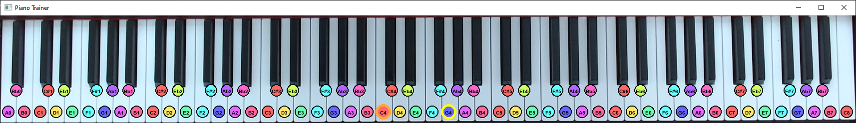
With the x-coordinates of each key identified, I labeled them from A0 to C8. Note names are drawn using PIL.

# Draw white keys
# Define white keys in order from A0 to C8 (88-key piano standard)
white_keys = [
    'A0', 'B0',
    'C1', 'D1', 'E1', 'F1', 'G1', 'A1', 'B1',
    'C2', 'D2', 'E2', 'F2', 'G2', 'A2', 'B2',
    'C3', 'D3', 'E3', 'F3', 'G3', 'A3', 'B3',
    'C4', 'D4', 'E4', 'F4', 'G4', 'A4', 'B4',
    'C5', 'D5', 'E5', 'F5', 'G5', 'A5', 'B5',
    'C6', 'D6', 'E6', 'F6', 'G6', 'A6', 'B6',
    'C7', 'D7', 'E7', 'F7', 'G7', 'A7', 'B7',
    'C8'
]

# Define black keys (sharps/flats), skipping where there's no black key (e.g., between E and F)
black_keys = [
    "Bb0", "C#1", "Eb1", "F#1", "Ab1",
    "Bb1", "C#2", "Eb2", "F#2", "Ab2",
    "Bb2", "C#3", "Eb3", "F#3", "Ab3",
    "Bb3", "C#4", "Eb4", "F#4", "Ab4",
    "Bb4", "C#5", "Eb5", "F#5", "Ab5",
    "Bb5", "C#6", "Eb6", "F#6", "Ab6",
    "Bb6", "C#7", "Eb7", "F#7", "Ab7",
    "Bb7", "C#8"
]

# Indices in the white key list where black keys are positioned (for visual overlay)
black_key_indices = [
    1, 3, 4, 6, 7, 8, 10, 11, 13, 14,
    15, 17, 18, 20, 21, 22, 24, 25, 27, 28,
    29, 31, 32, 34, 35, 36, 38, 39, 41, 42,
    43, 45, 46, 48, 49, 50
]

# Convert the OpenCV image to a PIL image for easier drawing
cropped_pil = Image.fromarray(cv2.cvtColor(cropped_piano, cv2.COLOR_BGR2RGB))
draw = ImageDraw.Draw(cropped_pil)

# --- Draw white key labels ---
# Check that the number of key intervals matches the number of white keys
if len(xs_to_use) - 1 == len(white_keys):
    for i in range(len(xs_to_use) - 1):
        note = white_keys[i]
        # Calculate the midpoint between the current and next vertical key line
        mid_x = int((xs_to_use[i] + xs_to_use[i + 1]) / 2)
        # Draw the note label or marker at the midpoint
        draw_note_circle(draw, mid_x, note)

# --- Draw black key labels ---
for idx, note in zip(black_key_indices, black_keys):
    # Make sure the index is within bounds of the x positions
    if idx < len(xs_to_use) - 1:
        # Use the x position directly for black keys
        mid_x = int(xs_to_use[idx])
        draw_note_circle(draw, mid_x, note)

Section 2: Note Parsing

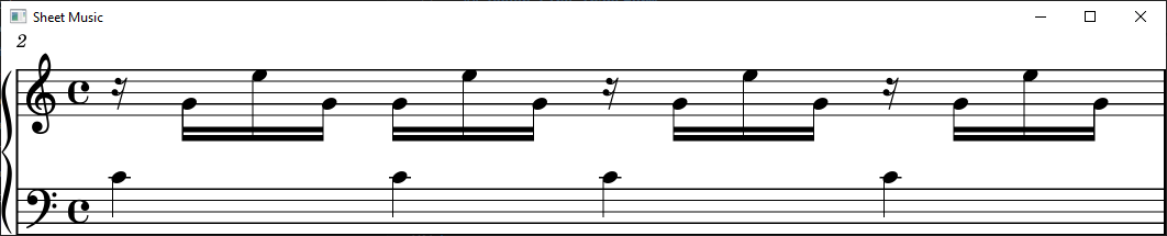
Sheet music in PDF format is converted to MusicXML using Audiveris, an open-source OMR tool. I parsed each bar, identify the notes, and highlight them on the keyboard: yellow for the treble clef (right hand), orange for the bass clef (left hand). The example below shows the fourth note in this bar highlighted on the keyboard. The accompanying code demonstrates how a MusicXML file is converted into a sequence of notes to be displayed on the keyboard labels for both hands.

def parse_sheet(filepath):
    # Parse the sheet music file into a music21 Score object
    score = converter.parse(filepath)

    # Map part indices to clef labels: 0 for treble, 1 for bass
    part_labels = {0: "treble", 1: "bass"}

    # Dictionary to group notes by their time offset (rounded), and store by clef
    # Each entry stores treble notes, bass notes, and the measure number
    grouped = defaultdict(lambda: {"treble": [], "bass": [], "measure": None})

    # Iterate over each part (e.g., treble and bass staves)
    for i, part in enumerate(score.parts):
        label = part_labels.get(i, f"part{i}")  # Label the part

        # Iterate through all notes and chords in the part
        for n in part.flat.notes:
            key = round(n.offset, 3)  # Use offset as grouping key, rounded for precision
            measure = n.getContextByClass("Measure")  # Get the measure the note belongs to
            mnum = measure.number if measure else 1   # Default to measure 1 if not found

            # If it's a single note, store its pitch with octave
            if isinstance(n, note.Note):
                grouped[key][label].append(n.nameWithOctave)
            # If it's a chord, store all its pitches with octave
            elif isinstance(n, chord.Chord):
                grouped[key][label].extend(p.nameWithOctave for p in n.pitches)

            # Save the measure number for this offset
            grouped[key]["measure"] = mnum

    # Convert the grouped dictionary to a sorted list of (treble_notes, bass_notes, measure)
    return [
        (entry["treble"], entry["bass"], entry["measure"])
        for offset, entry in sorted(grouped.items())
    ]

Section 3: Note detection

Spectrogram analysis and thresholding

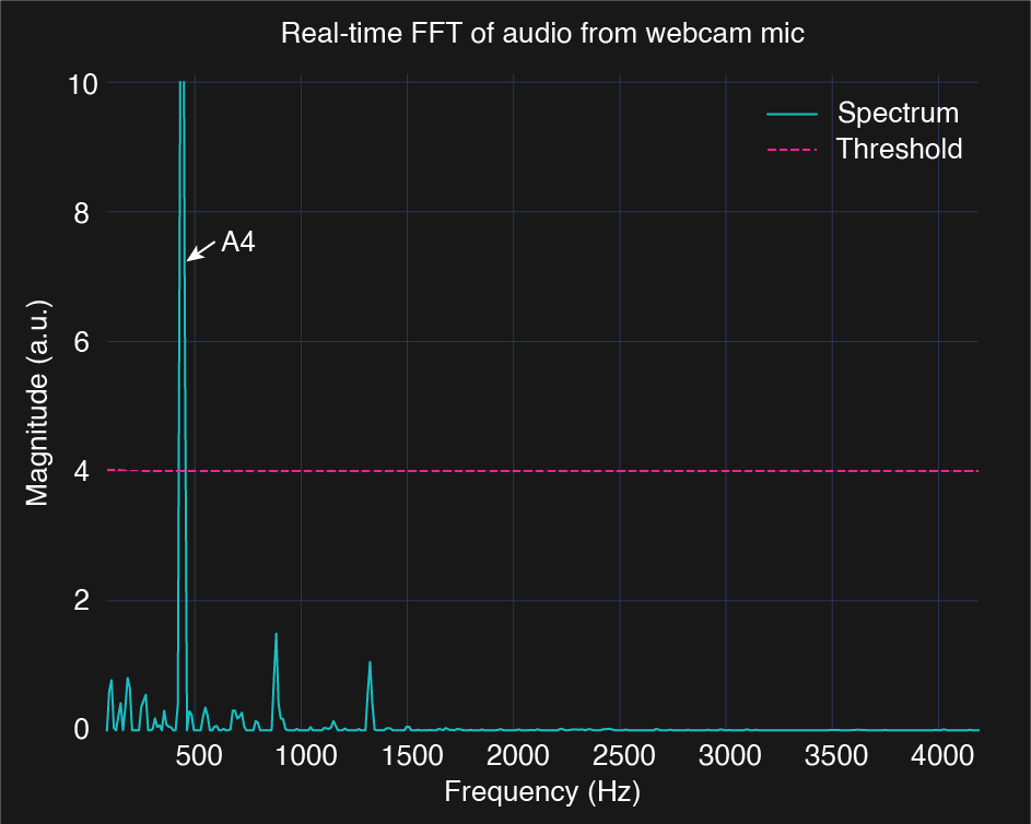
To detect which notes are played, I use the webcam’s microphone to capture audio and compute its spectrogram using FFT. A 3-second background spectrogram is first recorded to capture ambient noise, which is then subtracted from incoming frames.

The cleaned spectrum is scanned for frequency peaks. These are compared against the expected frequencies of piano notes, derived from the equal temperament system. A4 is defined as 440 Hz, and each semitone differs by a factor of \(\sqrt[12]{2}\). For example, the frequency of the 7th semitone above A4 corresponds to: \(f = 440 Hz \cdot 2^{\frac{7}{12}}\).

\[f = 440 \cdot 2^{\frac{n-69}{12}}\]

where:

\(f\) is the frequency of the note.
\(n\) is the MIDI note number.

The advantage of using MIDI note numbers is that both the pitch class (note name) and octave can be derived directly, where the note name is determined by \(n \bmod 12\) and the octave is given by \(\left\lfloor \frac{n}{12}\right\rfloor - 1\).

The image below shows the background-subtracted spectrum in real time as A4 is played. A threshold removes residual noise and harmonics. The 440 Hz peak is correctly identified as A4. If multiple peaks exceed the threshold, the system interprets them as simultaneous notes. The code shows how I convert a detected frequency into a note label such as “C4” or “A#5”.

def freq_to_note(freq):
    A4 = 440
    if freq <= 0:
        return None
    n = round(12 * np.log2(freq / A4)) + 69  # MIDI note number
    note_names = ['C', 'C#', 'D', 'Eb', 'E', 'F', 'F#', 'G', 'Ab', 'A', 'Bb', 'B']
    note = note_names[n % 12]
    octave = n // 12 - 1
    return note + str(octave)

Section 4: Video Demo

The first video demonstrates a simple single-note progression. It displays both the sheet music and a visual of the keyboard. As each bar is displayed in the score, the corresponding key is shown on the keyboard, guiding the player in real time. This showcases the system’s ability to assist with sight-reading and hand-eye coordination for beginners.

The second video highlights chord recognition. In addition to showing the sheet music and keyboard, it illustrates how the system waits for accurate input before progressing. If a wrong note is played—or if any note in a chord is missing—the playback does not advance. This feature reinforces correct playing and helps train precise chord execution.

Section 5: Limitation and What’s Next

Improving audio note detection robustness using better signal processing or machine learning.
Integrating PDF-to-XML conversion for a smoother workflow.
Adding dynamic note highlighting to the bar display.
Expanding hand tracking to suggest posture and position corrections.
Incorporating fingering suggestions, a valuable but challenging feature.

Icon credits: Input Icon: Kamin Ginkaew (Noun Project), Processing Icon: Deylotus Creative Design (Noun Project), Output Icon: Ian Rahmadi Kurniawan (Noun Project)